

National accounts and productivity estimates require measures of capital stocks, capital asset depreciation, and capital services.1 In the United States, the U.S. Bureau of Labor Statistics (BLS) constructs measures of capital services for its estimates of total factor productivity (TFP) growth for major sectors and detailed industries.2 The U.S. Bureau of Economic Analysis (BEA) develops estimates of economic depreciation, or consumption of fixed capital (CFC), that are used in constructing measures of net fixed investment (gross fixed investment less CFC), business income (such as corporate profits), and net saving. Estimates of stocks of fixed assets, net of CFC, appear in BEA fixed assets accounts and in balance sheets for major sectors in the integrated macroeconomic accounts.3
BLS and BEA use similar approaches to estimate capital stocks, building from BEA estimates of fixed investment, with different assumptions. Because the owners and users of productive capital are in most instances the same, no market data exist on rental prices of capital or the quantity of capital used. To estimate capital stocks and capital input, BLS and BEA combine data on investment, depreciation, and other volume changes, with assumptions about how efficiency declines with age. Capital stocks are estimated from data on investment and asset service lives. The capital input (also known as capital services) in each period is found by multiplying capital stocks by imputed rental prices, which are obtained from data on changes in asset prices and taxes combined with estimates of depreciation.
This article reviews recent research on depreciation rates and compares published BEA capital measures and BLS capital and TFP growth measures with simulated measures constructed by using alternative depreciation rates. The depreciation rates used by BEA and BLS for equipment and structures are mostly based on studies by Frank C. Wykoff and Charles R. Hulten.4 More recent studies by Statistics Canada estimated faster depreciation rates, especially for structures.5 These studies use Canadian data from Statistics Canada’s Annual Capital and Repair Expenditures Survey.6 This mandatory establishment survey collects data on sales and disposals of fixed assets, including asset type, gross book value, asset sales price, and age. A recent 2019 study of U.S. data by Sheharyar Bokhari and David Geltner also found faster depreciation rates for structures.7 In this article, we construct alternative estimates of BEA and BLS capital measures by using depreciation rates derived from the Statistics Canada data. Depreciation rates can differ across countries for many reasons, but the similarity of the results from Statistics Canada and Bokhari and Geltner suggests that the Statistics Canada rates can provide some useful insights for the United States. We present alternative estimates to test how the choice of depreciation rates matters for key statistics such as TFP, net capital stocks, and net investment and for international comparisons of these statistics.
Empirical studies of depreciation rates use the limited information available on used capital asset sales to capture depreciation rates of new and potentially improved capital assets, as well as changes in depreciation of existing capital assets. Depreciation is the decline in value of capital assets as they age and become less efficient in production because of wear and tear, increased maintenance requirements, obsolescence, accidental damage, and aging, including retirements.8 As explained by Barbara M. Fraumeni,9 “Obsolescence is a decrease in the value of an asset because a new asset is more productive, efficient, or suitable for production. A new asset might be more suited for production because it economizes on an input that has become relatively more expensive.” Depreciation rates reflect the effects of both physical deterioration and obsolescence and may vary over time because of changes in the characteristics of capital assets and their uses in production and because of changes in economic conditions, including tax and regulatory laws. Rapid improvement in semiconductor and computer technologies gives owners a stronger incentive to replace earlier vintages of goods with newer versions, such as smart phones that have taken the place of many earlier devices by incorporating computer, GPS, camera, flashlight, and other functions. The relevance of these technologically sophisticated goods has grown in the contexts of cloud computing, the Internet of Things, 3D printing, robotics, virtual reality, and autonomous vehicles.10 Manufacturing changes include smart factories capturing real-time data from sensors on machines, devices, and production systems to optimize production; improved industrial robots; and more agile automated production platforms that use, for example, innovations such as automated guided vehicles that can be reconfigured as production needs change, instead of fixed conveyer systems.11 For some capital assets, these changes speed up rates of depreciation and obsolescence and reduce service lives. For others, service lives lengthen as newer vintages are built better and retain productive value longer.12
BEA depreciation rates are based on numerous studies conducted over many decades.13 Although BEA measures of net stocks, net investment, and CFC are widely cited, economists have expressed concerns about slowdowns in net investment.14 A recent study used BEA fixed assets accounts to estimate trends in net investment and stocks of infrastructure assets.15 Following the 2008 financial crisis, the Data Gaps Initiative, led by the International Monetary Fund, has encouraged the development of sectoral accounts, such as the Integrated Macroeconomic Accounts, which present national balance sheets (including stocks of fixed assets) for key economic sectors. Possible biases in depreciation rates are also a concern in the context of the 2007–09 Great Recession and the slowdown in measured productivity growth.
In the next section, we describe the role of depreciation rates in estimates of BEA and BLS capital measures. Then we review the available studies of depreciation rates. And finally, we explain how we constructed alternative depreciation rates for U.S. capital stocks on the basis of the rates used by Statistics Canada and summarize the changes to the BEA and BLS capital measures that result from using these alternative rates. We refer to the official estimates by BEA and BLS as the “published” figures and compare them with our experimental estimates based on the services lives in the Statistics Canada data, which we call “simulated” estimates.
Capital stocks and rental prices
The input of a capital asset to productive output for a year is defined as its annual rental price multiplied by the productive capital stock of the asset. Before the role of alternative depreciation rates is considered, understanding the construction of each of these components may be helpful. This section describes the methods used by BEA and BLS to measure capital stocks and rental prices.
Capital stocks
Capital stocks are measured as indexes representing aggregates of equipment, structures, and other productive assets at a particular time. BEA and BLS use a method designed to produce annual indexes of capital stocks that correlate to how much output they will produce, as do statistical agencies in most Organisation for Economic Co-operation and Development (OECD) countries. This method, known as the perpetual inventory method (PIM) or vintage aggregation, combines past amounts of investment into productive assets with models of how they will decline in efficiency. The estimate of the flow of capital services provided in each period is modeled as the capital stock index multiplied by an annual rental rate.16
Under the PIM, productive capital stock at the end of a given period is a weighted sum of past investments, in which older investments are weighted less because they have declined in productive capacity.17 The capital stock is equal to the accumulated productive capacity of past investments net of any depreciation and can be thought of as the amount of new investment that would be required to produce the level of capital services produced by existing assets of all ages.
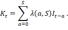
Let Kt denote the (net) productive capital stock of an asset type in year t, It–a denote investment expenditures in year t–a, where a indexes the ages of investments into the asset and t–a is called the vintage of each. Let S denote the maximum service life of the asset. Past investments are assumed to decline in productive capacity over time according to an assumed age-efficiency function, λ(a,S), which declines from 1 (when the asset is new) to zero (when a ≥ S) and represents the proportion of the investment’s original productive capacity that remains at age a. The productive capital stock of a group of assets with a maximum service life of S years is given by
 (1)
(1)
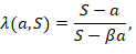
The age-efficiency function accounts for the decline in the productive capacity of the assets due to physical deterioration or obsolescence. Therefore, the rates at which the productive capacity of the assets decline have a key role in these capital measures. While investment data are available, detailed quantitative information on how the efficiency of capital assets declines over time is not. Implementing the PIM requires assumptions about how asset efficiency declines over time and when assets are retired. BLS assumes a hyperbolic age-efficiency function for an asset class,18 which is given by
 (2)
(2)
where λ(a,S) is the efficiency of an asset at age a relative to its performance when it was new; S is the asset service life; and β is a parameter that determines the shape of the age-efficiency function. When β is zero, an asset becomes less efficient, or deteriorates, by the same amount each year. When β is 1, the asset maintains the same level of efficiency until it reaches its service life, at which point it produces zero additional services. BLS uses a β value of 0.75 for structures assets and 0.50 for equipment assets.19 The λ(a,S) function models a slow initial decline in asset efficiency and a more rapid decline as asset age increases, a concave shape with respect to age.20 To account for the heterogeneity of asset service lives, BLS assumes that, within each asset category and cohort, service lives are distributed according to a modified normal distribution centered on the mean for that category. This cohort age-efficiency function is less concave than the function in equation (2). For most capital assets, BLS uses BEA depreciation rates to determine asset service lives that are consistent with the BLS hyperbolic age-efficiency function.21
An alternative approach to estimating capital stocks, a modified version used by BEA, is to assume a geometric pattern of depreciation.22 Under this assumption, the age-efficiency function becomes λ(a) = (1 – δ)a, where δ is the constant rate of depreciation and a is the age of the asset. Substituting λ(a) for λ(a,S) in the equation and rearranging terms, the PIM formula in equation (1) becomes
 (3)
(3)
The assumption of geometric depreciation means that the service life does not enter the age-efficiency function, the age-efficiency function of the asset is convex, and 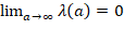 . An advantage of the geometric approach is that we do not need to track the vintages separately, but a disadvantage is that it imposes a convex aggregate age-efficiency shape regardless of the shape implied by the underlying empirical data.23
In addition to the assumption of geometric depreciation, BEA assumes that depreciation of current-year investment is one-half the annual depreciation rate, δ, because investment expenditures are distributed throughout the year.24 BEA also accounts for other events, Ot, such as losses due to disasters. The modified version of the geometric PIM for an asset is given by

(4)
The annual change in the net stock of an asset equals the additional investment minus the additional depreciation, as estimated by BEA using assumed asset-specific depreciation rates, destruction of capital from disasters, and other volume changes. Depreciation, Mt, is estimated as a residual. Rearranging from the expression,

(5)
BEA and BLS capital stocks are constructed from investment and service life data for similar categories of capital assets. BLS develops annual capital stocks that include 39 types of equipment assets, 32 types of private nonresidential structures assets, 11 tenant-occupied residential structures assets, 9 owner-occupied residential structures assets, 1 land asset, and 3 types of intellectual property assets. Intellectual property assets include software; research and development; and entertainment, literary, and artistic originals.25 BLS uses BEA data on gross investment expenditures by asset type for private U.S. businesses. Depreciation rates for each type of capital asset are calculated by using primarily BEA asset service lives and a hyperbolic age-efficiency schedule.
In summary, the stock of capital each year is modeled as the sum of past investments, net of depreciation. BLS capital stock measures are calculated from BEA gross fixed investment data by implementing the PIM with a hyperbolic age-efficiency function and BLS service lives estimated for most assets based on BEA asset depreciation rates.26 BEA measures of the market value of capital stock are based on accumulated fixed investment, net of depreciation. One difference between the BEA and BLS methods is that BEA assumes a geometric, rather than hyperbolic, pattern of depreciation.27 In practice, the BLS and BEA methods result in very similar depreciation rate and service life values for most capital assets.28
Rental prices
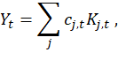
As just noted, BLS assumes that capital services in each period are proportional to the productive capital stock, in which the proportion is the rental rate of capital. BLS productive capital stocks, constructed for various types of capital assets, are aggregated by asset type, by using capital cost shares as weights. Implicit rental prices are calculated by assuming that the purchase price of a capital asset is equal to the discounted stream of services (and implicitly, the rents) that the asset will provide in the future. Laurits R. Christensen and Dale W. Jorgenson modeled price and quantity components of capital services by capital compensation, 29 which is equal to rental price multiplied by the productive capital stock, as
 (6)
(6)
where Yt is total capital income in year t, cj,t is the rental price of capital, Kj,t is productive capital stock, j represents the jth asset, and t represents the year t.
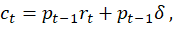
In a simplified equation that disregards inflation and taxes, the rental price for an asset may be given by
 (7)
(7)
where pt is the deflator for new capital goods, rt is the nominal rate of return, and δ is the average rate of economic depreciation.30 The rate of return rt is a percentage rate of return that represents the income that is generated per $100 of physical capital assets. The rental price measures the opportunity cost of using the asset. It reflects the income the business could have earned by loaning its financial resources in the debt market rather than investing in physical capital. From equation (7), we can see that the rental price is positively related to rates of return and depreciation. If the depreciation rates used are slower than the true rates, then BEA estimates of net investment, net stocks of fixed assets available for production, net saving, and corporate profits usually will be overestimated and CFC will be underestimated. Depreciation rates that are biased downward would lead to underestimates of the amount of depreciation for a given stock.31 The opposite biases in estimates of net stocks and depreciation will occur if the assumed depreciation rates are faster than the true rates.
The effect of underestimated depreciation rates on capital services and TFP is more complicated. Rates of return depend on the ratio of net capital income and the net capital stock, which is also affected by depreciation rates. One might expect that underestimating depreciation rates would lead to overestimating productive capital stock and capital services and, in turn, underestimating TFP. But there is an offsetting effect on capital rental prices. From equations (4) and (5), we can see that depreciation rates that are too low lead to lower rental prices and an underestimation of capital services. We examine the net impact of these two effects on the growth of capital services and TFP.
Both BLS and BEA capital measures rely on BEA estimates of fixed investment, and the definitions of investment are important for determining the relevant depreciation rate, especially for structures. Investment in private nonresidential structures is primarily based on value-put-in-place (VIP) data from the U.S. Census Bureau surveys of construction spending.32 The survey collects data on construction costs rather than the eventual selling price of the asset. The VIP measure includes the cost of new structures as well as modifications to existing structures, such as additions, renovations, and major replacements (a new roof, for example). It also includes installation of mechanical and electrical systems, such as plumbing, heating, elevators, and central air-conditioning equipment. It excludes the cost of land and the cost of routine maintenance and repairs. Depreciation rates for each of these components of structures may differ. Improvements and mechanical components may, for example, depreciate or become obsolete faster than the original “brick and mortar” building. Depreciation rates for each type of structure should reflect an aggregation of the depreciation rates of these components.33
Overview of research on depreciation
Although depreciation is an essential concept in economics, it is difficult to measure empirically, and different studies produce different estimates. Based on path-breaking studies of used asset transactions by Hulten and Wykoff, depreciation rates for structures and equipment used by BEA and BLS were developed primarily by Fraumeni.34 Recent studies by Statistics Canada and John Baldwin, Huju Liu, and Marc Tanguay, of Statistics Canada,35 based on used asset transactions in Canada from 1985 to 2010, applied methods similar to the Hulten and Wykoff methods and obtained generally faster depreciation (higher depreciation rates), especially for structures. Many other OECD countries use depreciation rates that are faster than the U.S rates. Although these studies raise questions about the U.S estimates, true depreciation rates may differ across countries for many reasons, so one should be cautious about applying rates from other countries to U.S. assets. But a recent study by Bokhari and Geltner,36 based on real estate transactions in the United States from 2001 to 2014, applied methods similar to the Hulten and Wykoff approach and also obtained faster depreciation rates for structures, similar to those found in the Statistics Canada studies. This section summarizes the data and methods used by these studies and discusses some key issues based on conversations with the authors and others who use these data.
The Hulten and Wykoff studies
The Hulten and Wykoff studies estimated depreciation patterns using samples of transactions of several types of used assets at market prices.37 For machinery and equipment, they acquired data on machine tools, construction machinery, autos, and office equipment from a variety of sources.38 For nonresidential structures, they used a sample of 8,066 observations of 22 types of buildings collected by the U.S. Department of the Treasury, Office of Industrial Economics (OIE), in 1972.39 For this sample, the owner of a building was asked when it was constructed, when the owner acquired it, and the price paid for it exclusive of the value of the land. With these data, Hulten and Wykoff could determine market transaction prices by age and date of purchase.40
Hulten and Wykoff used these data to estimate age-price profiles for those assets that were included in the OIE sample.41 Their estimation methods featured two key innovations. First, they made no assumption about the form of these profiles and used a flexible Box–Cox transformation instead to test whether the patterns resembled straight line, concave, or convex patterns. Second, because used asset prices reflect only surviving assets (a censored sample problem), Hulten and Wykoff weighted the used asset prices by the probability of survival before estimating the depreciation patterns. These weighted used asset prices thus reflect surviving and retired assets. The probability of survival depended on the mean and distribution of the service lives of assets. Service lives were based on the Department of the Treasury’s “Bulletin F,” and the distribution of retirements followed a Winfrey distribution.42
Hulten and Wykoff found that for most assets in their samples, the estimated age-price profiles were similar to a geometric (convex) form, with price declining more quickly early in the life of the asset before gradually diminishing to zero.43 With a geometric form, age-price profiles can be approximated by using a single constant rate of depreciation, a feature that simplifies computations of net stocks. Based on their estimated age-price profiles, Hulten and Wykoff produced estimates of depreciation rates for the assets in their samples. This set of assets, which they labeled “type A assets,” made up 55 percent of investment in equipment and 42 percent of investment in nonresidential structures in the National Income and Product Accounts (NIPA) in 1977.
To produce estimates of depreciation for the NIPA assets not included in the OIE sample, Hulten and Wykoff analyzed each asset on a case-by-case basis.44 These assets were then classified as either “type B” or “type C,” depending on whether empirical evidence was available regarding the depreciation pattern of the asset. The Hulten and Wykoff rates for both type B and C assets were based more on judgment than evidence. Depreciation rates for assets labeled type B were supported by data from existing empirical studies conducted by others as well and by using information available at the time on the treatment of depreciation by BEA, Dale Jorgenson, and Jack Faucett Associates.45 Little or no data were available for type C assets, and rates were developed based on inferences from similar type A category assets, where possible. Hulten and Wykoff assumed the depreciation pattern for these other assets was also geometric. To estimate depreciation patterns for the type C assets, Hulten and Wykoff used the relationship between the geometric depreciation rate (δ), the service life (S), and the declining balance rate (R) as

(8)
The value of the declining balance rate determines the shape of the depreciation pattern minus the extent to which asset values fall more rapidly early in the lifecycle.46 Higher values of R imply higher reductions in asset value earlier in the service life and more convex (such as geometric) depreciation profiles. For the assets for which data were available, Hulten and Wykoff estimated R values of 1.65 for equipment and 0.91 for nonresidential structures.47 These estimates contrast with an R value of 2.00 (double-declining balance), a rate often assumed by accountants to allow taxpayers to write off more depreciation expenses in the earlier years of asset ownership. Use of a double-declining balance rate for accounting purposes typically does not reflect the true decline in the efficiency of the assets. Hulten and Wykoff then estimated geometric depreciation rates for type C assets by dividing these declining balance rates by the existing estimates of service lives.
The Hulten and Wykoff studies became the standard, and subsequent studies used a similar method to estimate depreciation.48 In 1996, BEA released estimates of depreciation rates based largely on the Hulten and Wykoff studies.49 These updated depreciation estimates replaced previous estimates that were generally based on straight-line depreciation, by using available service lives, and Winfrey retirement patterns.50 For structures, the updated depreciation rates based on the Hulten and Wykoff studies were slower than the previous estimates and led to lower estimates of depreciation and higher estimates of net capital stocks. With few exceptions, BEA continues to use these rates for estimates of CFC and net stocks of nonresidential structures and equipment.51
Statistics Canada studies
Statistics Canada studies, like the Hulten and Wykoff studies, estimated depreciation patterns using samples of used asset transactions.52 Both sets of studies employed flexible specifications to test the shape of the age-price pattern (straight line, concave, convex, etc.), experimented with alternative assumptions regarding the retirements and discards, and estimated values of structures net of land values.
The data used for the Statistics Canada studies are based on their Annual Capital and Repair Expenditures Survey.53 The survey provides detailed information on asset type, gross book value, sale price, and age of each asset that is sold or discarded. The gross book value includes the original investment value plus the capitalized improvements over the life of the asset. Investment deflators were used to express all data in constant prices. The data in the 2007 Statistics Canada study cover the period from 1985 to 2001 (30,350 observations and 43 assets), and the 2015 Statistics Canada study extends the sample to cover the period from 2002 to 2010 (an additional 22,129 observations on 32 assets). These studies cover a more recent period and use larger samples of a wider range of assets than the Hulten and Wykoff studies.54 The Statistics Canada studies also include data on the ages of discarded assets and on the value of capitalized improvements, whereas the Hulten and Wykoff studies use market transaction prices to reflect the remaining present value of capital assets because these prices are affected by discards and capitalized improvements.55
The Statistics Canada researchers edited the survey data to screen and adjust outlier observations that seemed unrealistic. Some sale prices close to zero were classified as discards.56 Some long-lived assets that sold close to their original purchase price were excluded from the sample.57 When reported asset durations were concentrated on rounded values like 5, 10, and 20 years, the authors employed a correction to apply a distribution to the rounded values. The estimates were limited to those assets with active resale markets.
The key variable in the Statistics Canada studies is the ratio between the asset price when sold (SV) and its gross book value (GBV), SV/GBV, where both numerator and denominator are expressed in constant prices.58 Using this ratio and the age of the asset when sold, the studies estimated an age-price relationship that can be converted to a depreciation profile. The Statistics Canada studies jointly estimated asset survival and decline in value and the discard function using a flexible Weibull distribution that controls for price changes and other factors. They confirmed that the depreciation profiles generated by these econometric techniques produced convex age–price curves, consistent with geometric depreciation. The Statistics Canada studies also confirmed that the estimated depreciation rates changed little over the years in the sample.
A novel feature of the Statistics Canada studies was their comparison of these rates (“ex post rates”) and the anticipated length of service life reported by survey respondents for initial investments (“ex ante rates”).59 The Statistics Canada studies used these service lives and the declining balance rates obtained from their econometric analysis of depreciation to estimate alternative depreciation rates. The two sets of depreciation rates were generally very similar.
For many assets, especially structures, the Statistics Canada studies estimate faster depreciation than do the Hulten and Wykoff studies. The Hulten and Wykoff studies estimate an average rate of depreciation for structures of 3.7 percent, with a range of 1.9 percent to 5.6 percent, whereas the Statistics Canada studies estimate 6 percent to 8 percent.60 The declining balance rates from the Statistics Canada studies were generally 2 or higher, in contrast to the declining balance rates in the Hulten and Wykoff studies, which were below 2; higher declining balance rates imply more rapid depreciation earlier in the life of an asset. Both sets of studies used the available declining balance rates and data on service lives to estimate depreciation rates for some remaining assets. In its Measuring Capital manual, the OECD concluded, “This underlines the need for comprehensive and regular studies on depreciation patterns, lest there be a danger of ending up with biased values for depreciation and capital inputs.”61
Studies from other countries
The Economic and Social Research Institute, Cabinet Office, Government of Japan, initiated the Survey on Capital Expenditures and Disposals (CED) in 2006.62 The CED consists of three questionnaires focused on capital and repair expenditures, financial leases, and disposals. The CED has a detailed classification for more than 600 types of assets. In the disposal survey of the CED, assets are classified into four broad asset groups: buildings and accompanying equipment, machinery and equipment, transportation equipment, and other equipment. For each of these 4 asset groups, 15 observations of disposed assets, randomly selected by corporations, are reported, yielding a total of 60 observations of disposed assets covering all 4 asset groups if a firm fully responds. From these survey data, Japan’s Economic and Social Research Institute estimates depreciation rates and average service lives. In general, depreciation rates are found to be similar to the rates estimated by Statistics Canada and are faster than those used in the United States.63
Statistics Netherlands has estimated depreciation rates and service lives based on direct capital stock observations. In a study by Myriam van Rooijen-Horsten, Dirk van den Bergen, Ron de Heij, and Mark de Haan, the capital stock survey data were supplemented with discard data collected from an annual Survey on Discards.64 The study was conducted for all enterprises in the manufacturing industry with 100 or more employees and with annual Investment Survey data on additions to the capital stock in manufacturing industry enterprises with 20 or more employees. Combining data from the capital stock survey, discard survey, and investment surveys, the authors present estimated service lives for six asset categories by manufacturing industry: industrial buildings, civil engineering works, external transport equipment, machinery and equipment and internal means of transport, computers, and other tangible fixed assets. On the basis of the estimated depreciation rates and service lives, the authors of the study concluded that the discard survey may have missed a substantial portion of discards and that care needed to be taken in identifying reliable results. They also found the service life of an asset varied substantially depending on the manufacturing industry using the asset. Industry-specific service lives are developed by type of capital asset for NACE (Nomenclature of Economic Activities) two-digit-level industries. Because they assume different functional forms of depreciation, comparing their overall rates of depreciation with U.S. rates is not easy.
A 2016 Eurostat and OECD study reported on depreciation rate assumptions used by several national statistical agencies to estimate net stocks of structures.65 Canada, Japan, the Netherlands, and about two dozen other countries responded to the survey. Consistent with the studies just discussed, the study found that U.S. statistical agencies assume slower depreciation rates than do most OECD countries.
Depreciation rates from another country may not suit the United States because true depreciation rates vary across countries for many reasons. Differences in the mix and scale of industries, relative prices of capital and labor, capital utilization, economic and financial conditions affecting investment, tax policies, and climate across countries may affect capital asset depreciation rates. Depreciation rates for structures reflect differences in building standards and land-use regulations.66
Bokhari and Geltner study
A study by Bokhari and Geltner applied the Hulten and Wykoff method to a large sample of over 100,000 commercial real estate transactions in the United States from 2001 to 2014 and also found faster depreciation rates for structures, consistent with the Statistics Canada studies.67
The Bokhari and Geltner study used three data sets. The first data set, from Real Capital Analytics (RCA), consisted of transaction prices and other data from commercial and apartment property transactions, making possible estimation of property values or age profiles. The RCA data did not include information on investment in improvements, which BEA and BLS also capitalize.68 The other two data sets in the Bokhari and Geltner study measured investment in improvements. Data from the National Council of Real Estate Investment Fiduciaries (NCREIF) included over 15,000 properties (apartments, office, retail, and warehouses), with detailed information on rents and operating expenses, and separately identified capital improvement expenditures. Bokhari and Geltner write that their capital expenditures data include “only routine capital improvements and upkeep of the type that almost all commercial building owners must undertake on a regular basis (roof replacement, painting, carpeting, new appliances, new HVAC systems, landscaping, tenant custom fit-outs, etc.”)69 Thus, the data omitted major renovations and understated total investment in improvements. Data from Green Street Advisors on capital improvement expenditures for 1,299 apartment properties owned by real estate investment trusts were used to corroborate the findings from the NCREIF data set.70
The Bokhari and Geltner study defined “gross depreciation” as the sum of “net depreciation” (the depreciation of the original structure) plus capital improvement expenditures.71 Bokhari and Geltner illustrate the significance of this definition by using the following example: “. . . suppose a property with a 10-year-old building has market value of $100, and an otherwise identical 11-year-old property has market value of $97 as of the same time. Now suppose that during the previous year the owner of the 11-year-old building put $1 of capital improvement into the building, increasing its market value to $98. (This $1 of capital improvement expenditures would have to some extent mitigated the wear and tear and the functional obsolescence of the building.)”72 “. . . our estimated value/age profile based on our transaction price data would show 11-year-old properties selling for only 2 percent less than 10-year-old properties, even though the total capital consumption occurring between age 10 and 11 is 3 percent of the property value.” As the authors state, “this example illustrates why we need to separately estimate the cost of capital improvements and add that cost to the net depreciation that we observe in our empirically estimated value/age profile, in order to quantify total capital consumption.”73
To estimate net depreciation using the RCA data, Bokhari and Geltner used methods generally similar to those in the Hulten and Wykoff studies.74 They regressed the log of the expected price (the actual price times the survival probability) on age dummy variables, location characteristics, and a set of year dummy variables to control for factors such as changes in land and construction prices. The coefficients of the age dummy variables provided a nonparametric estimate of a depreciation pattern that is nearly geometric for nonresidential and apartment buildings. The authors also removed the effects of land values from their estimated depreciation rates by using their estimates of the share of land in the total property value. Their estimated net depreciation rates were 3.1 percent for nonresidential structures and 3.9 percent for apartment structures, higher than the Hulten and Wykoff estimates.75
The Bokhari and Geltner study then used the NCREIF data to estimate patterns of capital improvement expenditures by age.76 They regressed annualized capital improvement expenditures as a share of the market value of the building on age, age squared, and several controls for building characteristics. They found that capital improvement expenditures as a fraction of property value tended to increase over much of the lifespan of the property (and they may be underestimating capital improvement expenditures). The gross depreciation rate was calculated by using estimates of net depreciation and capital improvement expenditures. For a 25-year-old building, their estimate of gross depreciation was 6.61 percent for nonresidential buildings (3.14-percent net depreciation plus 3.47 percent for capital improvement expenditures) and 7.30 percent for apartments (3.94-percent net depreciation plus 3.36 percent for capital improvement expenditures). These gross rates of depreciation are close to those measured by the Statistics Canada studies.
Summary
The Statistics Canada and Bokhari and Geltner studies used the Hulten and Wykoff methods with recent data samples of used asset transactions and found faster depreciation than the Hulten and Wykoff studies, especially for structures. Possible explanations for these conflicting findings were discussed with the authors of the Hulten and Wykoff, Statistics Canada, and Bokhari and Geltner studies as well as users of BEA and BLS data at the Federal Reserve and other agencies. Overall, the authors remained confident in their own results and expressed some concerns about the other studies. Some of the capital specialists providing comments expressed concerns about using depreciation rates from other countries, because true depreciation rates could differ across countries for many reasons, although the Statistics Canada and Bokhari and Geltner estimates were similar. All were sympathetic to efforts to update research on the depreciation rates currently used by BEA and BLS. Regarding future updates of depreciation rates, the general recommendation was to proceed cautiously, given the numerous challenges in estimating depreciation. Some experts recommended BEA and BLS begin a new program of studies to develop updated rates by using the Hulten and Wykoff methods and new data. However, developing appropriate data sets of used asset transactions is difficult and demanding. There are active global markets for many types of used capital investment goods, including truck tractors, hydraulic excavators, dozers, backhoes, mobile cranes, machine tools, and conveyor belts. In principle, statistical agencies could therefore gather market prices for numerous specific types of used assets.77 However, considerable resources would be required to gather these data and develop contemporary depreciation rates for each asset type.
One of the key differences between these studies is how they incorporate data on improvements. Since the BEA estimates of fixed investment in structures include the cost of the original structures and subsequent improvements, depreciation rates for the capital stock also reflect depreciation of these improvements. The Bokhari and Geltner and Statistics Canada studies include data on improvements, while the Hulten and Wykoff studies do not. The Bokhari and Geltner study finds that improvements make up a substantial share of investment in structures. As the Bokhari and Geltner study points out, the omission of data on improvements may bias downward the estimate of cumulative investment in a structure and, given initial and subsequent sale prices of the building, may bias downward the estimate of total depreciation.78 In the Hulten and Wykoff studies, the effect of (unmeasured) improvements would be reflected in the resale price of the building, but the total investment in the building prior to resale, and perhaps total depreciation, may be understated.79 Improvements such as wiring, heating and cooling, and renovations may experience depreciation and obsolescence at rates different from the original structure. Uncertainty exists about how well the data on improvements in the Statistics Canada and Bokhari and Geltner studies measure investment that should be capitalized and depreciated. It is difficult to differentiate in the data between “improvements” that should be capitalized and “maintenance and repairs” that should not. Still another question is whether the respondents to the U.S. Census Bureau construction surveys (the basis for BEA estimates of investment) fully and accurately report these improvements, although the U.S. Census Bureau questionnaires clearly request these data.
Other considerations include a range of issues about the methods and conclusions of these studies. For the Statistics Canada studies, questions were raised about the econometric specifications, the price measures used, and reporting problems with their survey data. For example, firms might report expected service lives as round numbers or numbers developed for tax purposes rather than based on actual observation. The authors of the Statistics Canada studies did not share these concerns and questioned some details about the Hulten and Wykoff studies. For example, they expressed concern that the data on building prices may have included the value of land, resulting in unrealistically low estimated declining balance rates. The building price data used in the Hulten and Wykoff study were obtained from U.S. Department of the Treasury surveys of building values, conducted in 1972 and 1973.80 These surveys asked building owners to provide “cost or other tax basis of property (less land),” among other items. To the extent that building owners responding to these surveys complied with this direction, the Hulten and Wykoff building price data exclude the value of land.
One difficulty in comparing across studies is that depreciation rates are not necessarily stable over time. For example, when fiber optics were adopted for communication networks, copper wire telephone networks were replaced as a whole. That event caused sudden obsolescence, that is, faster depreciation for a brief time.
Simulation of U.S. capital accounts using Canadian service life data
In this section, we consider the potential impact of using alternative depreciation rates on several key BEA and BLS capital measures. We use Statistics Canada data on equipment and structures and assume that fixed asset depreciation and economic and technological trends are broadly similar in the U.S. and Canadian economies.
Asset service lives may differ because of country-specific factors such as variations in capital utilization, relative prices of capital and labor, economic and financial conditions affecting investment decisions, and climate.81 The secondary market for productive assets may also differ substantially between countries, for example, because of tax differences. These factors could lead to different sale and discard prices in the two countries and different efficiency curves and depreciation rates.
However, the similarity of results from the Statistics Canada studies and the recent Bokhari and Geltner study, which only includes U.S. data on structures, suggests that the Statistics Canada rates are plausible proxies for the United States. Our goals are to describe the potential impact of using the Statistics Canada or Bokhari and Geltner rates in BEA and BLS capital measures, to enable cross-national comparisons of these outcomes, and to encourage further research on depreciation rates.
We developed a concordance between the asset classification systems of the two countries. Statistics Canada uses an asset classification system that features more detailed asset categories in general than the U.S. asset classification system.82 While some asset categories are direct matches, other categories include more detailed assets in the Canadian system.
An example of a direct match between the Canadian and U.S. asset classification schemes is the BLS category autos (asset 22), which has a depreciation rate of 0.2165, and the Canadian category passenger cars (asset MPG336111), which has a faster depreciation rate of 0.2990. The U.S. category medical equipment and related instruments (asset 27) is classified as a direct match with the Canadian category medical, dental and personal safety supplies, instruments and equipment (asset MPG339100), which has more than double the published U.S. depreciation rate, at 0.301.
In most cases, the asset categories are similar but do not match exactly. We carefully reviewed the categories to match the Canadian asset categories to the U.S. asset categories on the basis of a detailed study of each asset description. This matching process typically resulted in a combination of Canadian asset categories being related to a single broader U.S. asset category. For example, the U.S. asset category other fabricated metal products (asset 3) corresponds to five detailed Canadian asset categories. A new depreciation rate for the broader U.S. asset category was developed by weighting the depreciation rates for the more detailed Canadian categories with the use of detailed nominal investment data from BEA benchmark (economic census year) estimates.83
In a few instances, to build up the underlying asset detail matches to the U.S. broader categories, we assigned a detailed Canadian asset category to multiple U.S. asset categories. For example, the BLS steam engines and turbines (asset 4) category is matched with the Statistics Canada category turbines and turbine generator set units (asset MPG333601). The BLS category internal combustion engines (asset 5) is also matched with turbines and turbine generator set units (asset MPG333601), as well as other engine and power transmission equipment (asset MPG333609). This matching was done selectively, in those instances in which the Canadian category—while not a perfect match—was the best match to detailed assets in more than one U.S. fixed investment expenditure category. In the case of internal combustion engines (asset 5), the investment weighted depreciation rate becomes 0.0929 rather than the BLS value of 0.1972. This asset is one of the few for which the service life obtained from Canadian data is greater than the published U.S. value.
The published U.S. asset classification scheme includes a few assets in which the service lives depend on industry of use. For example, the U.S. classification scheme includes different depreciation rates for 22 industries under the asset category metal working machinery (11). These service lives range from a low of 12 years in North American Industry Classification System (NAICS) code 321, wood products industry, to a high of 28 years in NAICS code 331, primary metal manufacturing industry. Special industry machinery (12) and general industrial equipment including materials handling (13) also have multiple service lives based on the industry in which the asset is used. These industry-specific depreciation rates for selected asset categories were developed on the basis of industry studies conducted during the 1970s by the former OIE of the U.S. Department of the Treasury and from industry studies conducted during the 1980s and 1990s by the Office of Tax Analysis of the U.S. Department of the Treasury.84 To obtain revised depreciation rates for these asset-industry breakouts beneath assets 11, 12, and 13, we first noted that each of these three assets included industry-specific depreciation rates for 21 specific manufacturing industries and also for the nonmanufacturing industry category. For each of these three assets, we used the relationship between the depreciation rates for each specific industry and the nonmanufacturing industry category to adjust the Statistics Canada depreciation rate for the overall asset category.85 Generally, we found that the concordance of the U.S. and Canadian asset categories provided a reasonable scaffold on which to develop experimental depreciation rates for this analysis.
Using the asset category concordance, Canadian asset service lives, and Canadian declining balance rates, we conducted two simulations with different sets of service lives.86 For the “set 1” simulation, we estimated new depreciation rates for 38 of the 39 U.S. equipment categories, all 32 private nonresidential structures categories, and 9 of the 11 tenant-occupied residential structures categories.87 Where a U.S. asset category was matched to multiple more detailed Statistics Canada assets, an overall depreciation rate was developed as a weighted average of the Statistics Canada depreciation rates, in which the weights used are the shares of 2007 U.S. fixed investment in the more detailed assets. Table 1 summarizes the published BEA and BLS depreciation rates and our set 1 alternative rates, derived from Statistics Canada data, for each U.S. asset category. (See source data under related content.) For most categories of equipment, the rates from Statistics Canada are higher, implying a faster rate of depreciation. Only three U.S. equipment asset categories have slower revised depreciation rates than published U.S. rates:
1. Asset 5: internal combustion engines
2. Asset 19: other electrical equipment
3. Asset 21: other trucks, buses, trailers in the transit and ground passenger transportation industry
For structures, the depreciation rates from Statistics Canada are typically faster. For many types of buildings, the published BEA and BLS depreciation rates are in the range of 2 percent to 3 percent, whereas the alternative Statistics Canada based estimates are 6 percent to 8 percent.
To obtain revised service lives from the set 1 depreciation rates, we assumed a geometric age-efficiency function and used the relationship between the depreciation rate and the ratio of the declining balance rate to the service life as described in equation 8. We combined the Statistics Canada-derived depreciation rates in set 1 with BEA declining balance rates to obtain the corresponding set 1 service lives for each U.S. asset category, on the basis of the use of a geometric age-efficiency function. For the BLS simulations, these revised set 1 service lives were adjusted to equivalent hyperbolic age-efficiency function service lives, and the associated depreciation rates were calculated.
We also used the Canadian data to estimate a second simulation of depreciation rates, “set 2.” Rather than using weighted averages of the Canadian depreciation rates to obtain rates for U.S. assets, we combined data on U.S. service lives with Statistics Canada declining balance rates. Using this approach allowed us to retain some of the information from historical U.S. studies of average service lives and to investigate the effect of more recent findings of Statistics Canada on the pattern of depreciation over time. For each U.S. asset category, we constructed estimates of declining balance rates from Statistics Canada data using our concordance between the U.S. and Canadian capital asset classification systems. The Statistics Canada declining balance rate value for each U.S. asset was divided by the BEA service life for each asset to obtain a revised depreciation rate. We then estimated the effect of the set 2 depreciation rates on BEA and BLS capital measures and BLS TFP measures.
In general, the set 2 depreciation rates fell between those in set 1 and the published BLS and BEA rates. Table 2 provides a more detailed comparison of the published and revised depreciation rates and service lives. (See source data under related content.)
When assessing the results of these simulations, note that the values of BLS and BEA capital stock measures are not directly comparable for several reasons. BLS capital stocks are consistently higher than BEA capital stocks in part because BLS uses a hyperbolic age-efficiency function, which retains capital assets in capital stock for a relatively longer time than the BEA geometric depreciation function. Also, BLS capital stocks include land and inventories, while BEA fixed assets accounts do not. BLS also has relatively higher estimates of stocks of structures, equipment, and intellectual property products because BLS uses slower depreciation rates for some types of assets and because BLS and BEA use different functional forms for depreciation. BEA and BLS estimate capital stocks for different purposes: BEA estimates the market or replacement value of stocks for national accounts and balance sheets, whereas BLS estimates the value of productive capital and its capital services.
Simulation of capital measures using the revised service lives
To describe the potential effect of using these alternative depreciation rates, we substituted the revised rates into the BEA and BLS PIM and rental rate calculations to estimate simulated capital stock and capital services measures. We estimated our capital measures using both the set 1 and set 2 depreciation rates. In each simulation, we maintained the existing depreciation rates through 1984 and introduced the revised rates for all assets beginning in 1985. This approach simulated changing depreciation rates by assuming that the newer Statistics Canada rates are more appropriate for later years, whereas the published BEA and BLS rates are more appropriate for earlier years. Real depreciation rates most likely change gradually.
BEA-simulated capital measures
The use of the faster depreciation rates from Statistics Canada resulted in an upward revision to estimates of CFC (consumption of fixed capital), relative to BEA published estimates. (See chart 1.) Under the set 1 simulation, which implements revised rates starting in 1985, CFC is revised upward by $308 to $170 billion annually for 1985–94, $170–$214 billion for 1995–2004, and $222–$249 billion for 2005–18. When the generally slower depreciation rates from set 2 are used, CFC is revised upward by $206–$125 billion annually for 1985–94, $125–$163 billion for 1995–2004, and $168–$195 billion for 2005–19. In most years, the upward revision to CFC is larger for structures than for equipment because differences in depreciation rates and the capital stocks are larger for structures. (This detail is not shown in the chart.) As a percentage of the published CFC values, the upward revision to CFC declines from about 25 percent in 1994 to about 11 percent in 2019 (set 1) and declines from about 19 percent in 1994 to 8 percent in 2018 (set 2). Faster depreciation rates result in upward revisions to CFC that decline in percentage terms over time because the faster depreciation rates also result in downward revisions to net stocks. These lower net stocks lead to a partly offsetting decline in estimates of CFC. The notable upward revision to depreciation in 1985 results from our abrupt introduction of new rates in that year. A gradual transition in which rates were slowly revised upward over several years before 1985 is more realistic.
| Year | BEA | Set 1 | Set 2 |
|---|---|---|---|
|
1985 |
$403.65 | $711.67 | $609.78 |
|
1986 |
430.63 | 706.51 | 617.00 |
|
1987 |
455.98 | 703.51 | 623.00 |
|
1988 |
489.84 | 719.74 | 648.07 |
|
1989 |
523.79 | 741.26 | 675.81 |
|
1990 |
556.86 | 762.94 | 702.80 |
|
1991 |
585.88 | 778.20 | 723.86 |
|
1992 |
603.09 | 782.00 | 732.88 |
|
1993 |
629.54 | 801.84 | 755.94 |
|
1994 |
664.45 | 834.63 | 789.82 |
|
1995 |
713.36 | 883.57 | 838.22 |
|
1996 |
753.50 | 925.59 | 879.14 |
|
1997 |
802.95 | 979.07 | 930.63 |
|
1998 |
855.69 | 1,042.12 | 989.88 |
|
1999 |
920.75 | 1,123.46 | 1,065.64 |
|
2000 |
1,002.31 | 1,222.31 | 1,159.29 |
|
2001 |
1,063.18 | 1,290.34 | 1,225.71 |
|
2002 |
1,098.20 | 1,320.69 | 1,259.44 |
|
2003 |
1,125.07 | 1,338.86 | 1,282.83 |
|
2004 |
1,177.81 | 1,391.58 | 1,338.63 |
|
2005 |
1,264.29 | 1,485.82 | 1,432.59 |
|
2006 |
1,359.77 | 1,592.56 | 1,537.71 |
|
2007 |
1,447.24 | 1,690.10 | 1,633.94 |
|
2008 |
1,532.59 | 1,781.20 | 1,727.20 |
|
2009 |
1,547.38 | 1,783.79 | 1,739.01 |
|
2010 |
1,558.56 | 1,775.36 | 1,739.94 |
|
2011 |
1,624.35 | 1,836.22 | 1,804.04 |
|
2012 |
1,706.73 | 1,918.33 | 1,887.62 |
|
2013 |
1,778.76 | 1,992.96 | 1,961.76 |
|
2014 |
1,873.55 | 2,094.49 | 2,061.79 |
|
2015 |
1,947.74 | 2,175.49 | 2,137.63 |
|
2016 |
1,995.82 | 2,225.88 | 2,178.46 |
|
2017 |
2,078.96 | 2,312.80 | 2,257.46 |
|
2018 |
2,172.07 | 2,414.21 | 2,354.12 |
|
2019 |
2,285.30 | 2,537.54 | 2,473.34 |
These upward revisions to CFC lead to downward revisions to net stocks, as shown in chart 2. When the revised set 1 depreciation rates are used, net stocks (in current dollars) are reduced by $309 billion in 1985. This downward revision grew to over $10.4 trillion in 2018—a downward revision of 39.7 percent in current dollars. The downward revision to net stocks in 2018 is about $2.4 trillion for equipment and $8.0 trillion for structures. These downward revisions imply reductions in estimates of the value of fixed assets in the balance sheets of the business sector in the integrated macroeconomic accounts (sectoral accounts).88 When the set 2 depreciation rates are used, net stocks are reduced in 2018 by $8.0 trillion (30.4 percent).
| Year | BEA | Set 1 | Set 2 |
|---|---|---|---|
|
1985 |
$5,332.39 | $5,023.04 | $5,126.47 |
|
1986 |
5,603.64 | 5,010.10 | 5,211.11 |
|
1987 |
5,919.09 | 5,061.54 | 5,352.61 |
|
1988 |
6,311.27 | 5,189.81 | 5,561.85 |
|
1989 |
6,699.83 | 5,323.22 | 5,775.79 |
|
1990 |
7,071.32 | 5,447.48 | 5,970.35 |
|
1991 |
7,242.59 | 5,419.05 | 6,010.18 |
|
1992 |
7,487.03 | 5,454.37 | 6,106.16 |
|
1993 |
7,837.56 | 5,580.54 | 6,297.43 |
|
1994 |
8,272.94 | 5,774.62 | 6,558.88 |
|
1995 |
8,723.34 | 5,992.38 | 6,838.46 |
|
1996 |
9,152.35 | 6,199.88 | 7,104.99 |
|
1997 |
9,674.78 | 6,487.80 | 7,441.57 |
|
1998 |
10,226.57 | 6,836.65 | 7,854.06 |
|
1999 |
10,849.37 | 7,233.67 | 8,328.06 |
|
2000 |
11,608.76 | 7,716.11 | 8,884.68 |
|
2001 |
12,189.37 | 8,014.48 | 9,245.03 |
|
2002 |
12,615.89 | 8,175.90 | 9,456.14 |
|
2003 |
13,036.24 | 8,346.12 | 9,680.55 |
|
2004 |
14,150.50 | 8,920.08 | 10,351.19 |
|
2005 |
15,429.81 | 9,612.10 | 11,097.50 |
|
2006 |
16,707.30 | 10,323.48 | 11,896.98 |
|
2007 |
17,653.79 | 10,872.87 | 12,529.31 |
|
2008 |
18,787.12 | 11,486.88 | 13,234.87 |
|
2009 |
18,237.61 | 11,049.14 | 12,840.98 |
|
2010 |
18,684.48 | 11,195.84 | 13,039.81 |
|
2011 |
19,551.28 | 11,632.78 | 13,540.70 |
|
2012 |
20,216.93 | 11,992.77 | 13,943.04 |
|
2013 |
21,073.28 | 12,480.31 | 14,470.01 |
|
2014 |
22,037.14 | 13,067.24 | 15,074.15 |
|
2015 |
22,486.96 | 13,310.56 | 15,387.16 |
|
2016 |
23,118.30 | 13,657.65 | 15,807.76 |
|
2017 |
24,000.85 | 14,133.06 | 16,389.30 |
|
2018 |
25,219.99 | 14,824.72 | 17,250.48 |
|
2019 |
26,209.24 | 15,383.83 | 17,945.67 |
Downward revisions to net stocks reflect downward revisions to several categories of equipment and structures. Within equipment, downward revisions occurred for information processing equipment such as computers, communications equipment, and instruments ($0.6 trillion); industrial equipment ($0.9 trillion); transportation equipment ($0.4 trillion); and all other equipment ($0.5 trillion). Within structures, downward revisions occurred for commercial and healthcare ($3.2 trillion), manufacturing ($0.9 trillion), power and communication ($1.5 trillion), mining exploration ($0.6 trillion), and all other structures ($1.8 trillion).
As chart 3 shows, net investment is lower when simulated with the faster Statistics Canada depreciation rates, reflecting the upward revisions to CFC. These revisions to net investment do not shed any new light on the reasons for the timing of the productivity slowdown that began around 2004 because the capital simulations begin several years before the slowdown started. Nevertheless, the downward revisions to net investment and net stocks are noteworthy.89
| Year | BEA | Set 1 | Set 2 |
|---|---|---|---|
|
1985 |
$204.10 | $–103.92 | $–2.03 |
|
1986 |
177.13 | –98.74 | –9.24 |
|
1987 |
159.26 | –88.27 | –7.77 |
|
1988 |
172.44 | –57.46 | 14.21 |
|
1989 |
192.21 | –25.27 | 40.18 |
|
1990 |
182.37 | –23.70 | 36.43 |
|
1991 |
137.70 | –54.62 | –0.28 |
|
1992 |
138.85 | –40.06 | 9.06 |
|
1993 |
169.67 | –2.64 | 43.27 |
|
1994 |
204.40 | 34.22 | 79.03 |
|
1995 |
248.88 | 78.68 | 124.03 |
|
1996 |
289.70 | 117.60 | 164.06 |
|
1997 |
346.14 | 170.02 | 218.46 |
|
1998 |
398.45 | 212.03 | 264.27 |
|
1999 |
443.73 | 241.02 | 298.84 |
|
2000 |
496.13 | 276.12 | 339.14 |
|
2001 |
396.89 | 169.73 | 234.36 |
|
2002 |
254.65 | 32.16 | 93.41 |
|
2003 |
250.82 | 37.02 | 93.05 |
|
2004 |
289.56 | 75.79 | 128.74 |
|
2005 |
356.69 | 135.17 | 188.39 |
|
2006 |
434.03 | 201.24 | 256.09 |
|
2007 |
501.32 | 258.47 | 314.63 |
|
2008 |
458.28 | 209.67 | 263.68 |
|
2009 |
143.06 | -93.36 | -48.58 |
|
2010 |
176.42 | -40.38 | -4.96 |
|
2011 |
283.11 | 71.25 | 103.42 |
|
2012 |
411.80 | 200.20 | 230.91 |
|
2013 |
432.73 | 218.53 | 249.74 |
|
2014 |
526.50 | 305.57 | 338.27 |
|
2015 |
518.81 | 291.06 | 328.93 |
|
2016 |
464.68 | 234.62 | 282.04 |
|
2017 |
495.51 | 261.68 | 317.01 |
|
2018 |
604.58 | 362.44 | 422.54 |
|
2019 |
609.70 | 357.46 | 421.65 |
BLS-simulated capital measures
We used the revised depreciation rates to construct capital stock and capital services measures for major sectors, including the private business, private nonfarm business, and manufacturing sectors, and for 60 NIPA industries, roughly three-digit level, industries. Chart 4 presents the BLS official capital stock levels, in constant 2012 dollars, for the private nonfarm business sector along with the capital stock measures constructed with the use of the published BLS depreciation rates and the revised depreciation rates for both set 1 and set 2. The introduction of new rates in 1985 reduces the capital stock growth rate substantially over the 1987–2018 period, from the official value of 1.8 percent to 0.9 percent and 1.2 percent, for set 1 and set 2, respectively.
| Year | Official measure | Set 1 | Set 2 |
|---|---|---|---|
|
1987 |
$22,395.90 | $22,346.47 | $22,355.24 |
|
1988 |
22,938.20 | 22,824.10 | 22,846.38 |
|
1989 |
23,467.29 | 23,259.81 | 23,301.89 |
|
1990 |
23,978.30 | 23,648.29 | 23,716.22 |
|
1991 |
24,382.96 | 23,902.04 | 24,000.95 |
|
1992 |
24,685.42 | 24,028.36 | 24,162.07 |
|
1993 |
25,017.98 | 24,163.32 | 24,335.02 |
|
1994 |
25,406.10 | 24,334.93 | 24,548.41 |
|
1995 |
25,867.74 | 24,562.29 | 24,822.28 |
|
1996 |
26,359.65 | 24,803.03 | 25,115.98 |
|
1997 |
26,953.83 | 25,129.89 | 25,503.99 |
|
1998 |
27,644.02 | 25,537.00 | 25,981.64 |
|
1999 |
28,365.36 | 25,958.87 | 26,484.55 |
|
2000 |
29,137.56 | 26,415.15 | 27,033.77 |
|
2001 |
29,834.11 | 26,779.03 | 27,502.51 |
|
2002 |
30,326.57 | 26,924.45 | 27,761.95 |
|
2003 |
30,733.43 | 26,974.87 | 27,932.79 |
|
2004 |
31,164.48 | 27,044.81 | 28,126.51 |
|
2005 |
31,692.44 | 27,209.10 | 28,416.83 |
|
2006 |
32,309.81 | 27,458.52 | 28,793.79 |
|
2007 |
32,989.55 | 27,764.86 | 29,229.68 |
|
2008 |
33,623.12 | 28,017.68 | 29,613.67 |
|
2009 |
33,875.73 | 27,882.13 | 29,608.85 |
|
2010 |
34,002.04 | 27,622.08 | 29,473.43 |
|
2011 |
34,313.60 | 27,552.84 | 29,520.13 |
|
2012 |
34,760.97 | 27,626.42 | 29,700.89 |
|
2013 |
35,322.94 | 27,818.61 | 29,993.00 |
|
2014 |
35,986.30 | 28,113.90 | 30,382.24 |
|
2015 |
36,740.93 | 28,500.64 | 30,858.72 |
|
2016 |
37,425.58 | 28,815.97 | 31,262.30 |
|
2017 |
38,071.41 | 29,090.45 | 31,627.14 |
|
2018 |
38,813.33 | 29,458.33 | 32,090.34 |
Chart 5 presents annual growth rates of the BLS official capital stock for the private nonfarm business sector and the simulated capital stock measures based on published BLS depreciation rates for both sets 1 and 2.90 As just noted, BEA and BLS capital stock measures differ in terms of the assumptions made about asset depreciation rates and patterns of decline over time, as well as the types of assets included in each agency’s measures. Comparisons between the BEA and BLS capital stock measures as a result are somewhat problematic. Regardless, we see that the use of the Statistics Canada depreciation rates results in lower stocks for both sets of estimates.
| Year | Official measure | Set 1 | Set 2 |
|---|---|---|---|
|
1988 |
2.4 | 2.1 | 2.2 |
|
1989 |
2.3 | 1.9 | 2.0 |
|
1990 |
2.2 | 1.7 | 1.8 |
|
1991 |
1.7 | 1.1 | 1.2 |
|
1992 |
1.2 | 0.5 | 0.7 |
|
1993 |
1.3 | 0.6 | 0.7 |
|
1994 |
1.6 | 0.7 | 0.9 |
|
1995 |
1.8 | 0.9 | 1.1 |
|
1996 |
1.9 | 1.0 | 1.2 |
|
1997 |
2.3 | 1.3 | 1.5 |
|
1998 |
2.6 | 1.6 | 1.9 |
|
1999 |
2.6 | 1.7 | 1.9 |
|
2000 |
2.7 | 1.8 | 2.1 |
|
2001 |
2.4 | 1.4 | 1.7 |
|
2002 |
1.7 | 0.5 | 0.9 |
|
2003 |
1.3 | 0.2 | 0.6 |
|
2004 |
1.4 | 0.3 | 0.7 |
|
2005 |
1.7 | 0.6 | 1.0 |
|
2006 |
1.9 | 0.9 | 1.3 |
|
2007 |
2.1 | 1.1 | 1.5 |
|
2008 |
1.9 | 0.9 | 1.3 |
|
2009 |
0.8 | –0.5 | 0.0 |
|
2010 |
0.4 | –0.9 | –0.5 |
|
2011 |
0.9 | –0.3 | 0.2 |
|
2012 |
1.3 | 0.3 | 0.6 |
|
2013 |
1.6 | 0.7 | 1.0 |
|
2014 |
1.9 | 1.1 | 1.3 |
|
2015 |
2.1 | 1.4 | 1.6 |
|
2016 |
1.9 | 1.1 | 1.3 |
|
2017 |
1.7 | 1.0 | 1.2 |
|
2018 |
1.9 | 1.3 | 1.5 |
The change in service lives and depreciation rates is expected to reduce capital stocks, but the effect on capital services is less obvious. BLS measures of capital services are calculated as proportional to the capital stock, in which the proportion is the rental price of the asset.91 Capital services measures, in constant 2012 dollars, for the private nonfarm business sector under set 1 and set 2 scenarios and those for the BLS official measures are presented in chart 6. All set 1 and set 2 simulated capital services series values are greater than the official values during the first two-thirds of the time series. The official value of capital services starts lower than that of the other two series but surpasses those of the two set 1 capital services series by 2011. The trend lines for all three series are similar though, with relatively steady growth except for a slowdown during and following the Great Recession (December 2007 to June 2009).92
| Year | Official measure | Set 1 | Set 2 |
|---|---|---|---|
|
1987 |
$1,749.67 | $2,187.25 | $1,994.98 |
|
1988 |
1,815.95 | 2,255.72 | 2,065.40 |
|
1989 |
1,890.59 | 2,328.83 | 2,141.99 |
|
1990 |
1,955.46 | 2,384.97 | 2,199.27 |
|
1991 |
2,016.28 | 2,431.38 | 2,249.44 |
|
1992 |
2,068.20 | 2,465.60 | 2,291.60 |
|
1993 |
2,139.17 | 2,521.23 | 2,353.67 |
|
1994 |
2,220.24 | 2,590.20 | 2,427.45 |
|
1995 |
2,319.64 | 2,680.20 | 2,520.91 |
|
1996 |
2,430.46 | 2,783.09 | 2,626.32 |
|
1997 |
2,561.57 | 2,907.61 | 2,752.48 |
|
1998 |
2,718.64 | 3,059.49 | 2,906.70 |
|
1999 |
2,894.76 | 3,231.89 | 3,081.56 |
|
2000 |
3,081.97 | 3,412.78 | 3,266.29 |
|
2001 |
3,233.37 | 3,544.43 | 3,409.88 |
|
2002 |
3,344.06 | 3,623.64 | 3,507.37 |
|
2003 |
3,440.14 | 3,685.35 | 3,587.69 |
|
2004 |
3,534.21 | 3,749.12 | 3,666.58 |
|
2005 |
3,656.07 | 3,844.28 | 3,772.53 |
|
2006 |
3,793.11 | 3,959.91 | 3,895.02 |
|
2007 |
3,921.66 | 4,066.39 | 4,009.68 |
|
2008 |
4,035.13 | 4,152.91 | 4,108.48 |
|
2009 |
4,077.92 | 4,153.03 | 4,131.80 |
|
2010 |
4,108.95 | 4,134.08 | 4,136.58 |
|
2011 |
4,179.19 | 4,162.99 | 4,182.09 |
|
2012 |
4,262.40 | 4,210.89 | 4,241.28 |
|
2013 |
4,369.60 | 4,285.88 | 4,324.25 |
|
2014 |
4,492.61 | 4,378.20 | 4,422.52 |
|
2015 |
4,629.30 | 4,485.87 | 4,532.26 |
|
2016 |
4,766.43 | 4,592.37 | 4,638.63 |
|
2017 |
4,897.49 | 4,690.50 | 4,737.17 |
|
2018 |
5,036.19 | 4,796.09 | 4,844.53 |
The revised and generally faster depreciation rates used in our capital services simulations had little effect on the estimates of capital services. This outcome can be explained by the offsetting effects of faster depreciation rates on capital stock and capital services measures. Changes in depreciation rates directly affect both productive capital stock measures and rental price measures. Faster depreciation rates lead to increases in rental prices and capital services per dollar of stock, which offset the reduction in productive stocks. The net effect on capital services is small. However, rental prices also function as a means of allocating capital income among capital assets. A change in depreciation rates may result in a change in the productive capital stock measures by asset type as well. Therefore, simulated asset prices may alter the allocation of capital income among the assets by modifying the weights used to aggregate detailed capital assets into the broader capital stock measures.
Faster depreciation rates also have offsetting effects on rates of return and capital stocks in the corporate sector. This offsetting effect occurs because the BLS capital measurement method adopts BEA corporate capital income and total capital income as given. Only BLS noncorporate capital income changes relative to depreciation rates and rental price fluctuations. For example, a change in depreciation rates may change the distribution of proprietors’ income to labor and capital. Thus, the impact of changes in the depreciation rates on capital services would be minimal and reflect only changes in the distribution and weighting of assets and changes in noncorporate capital income.
Differences were substantial between the 1987–2018 annual growth rates of the BLS official capital stock measure and capital stock measures based on revised rates for 1985 forward by NIPA industry, with about a percentage-point difference for set 1 and slightly less for set 2. (See chart 5.) Similar effects are observed in chart 7 (which displays annual growth rates of capital services measures) for the BLS official capital services measure and the simulated capital services measures. Note that the updated capital services measures have very similar annual growth-rate movements, with level shifts that remain relatively consistent among the separate series. Again, with new service lives applied beginning in 1985, the growth rates of capital services series simulated by using set 1 and set 2 are lower than the published BLS series. For the major sectors, capital stock levels and growth rates are affected by the revised service lives. The reductions in the level of capital stock are expected given the generally downward revisions in service lives and upward adjustments in depreciation rates. On the other hand, little difference exists in capital services levels and growth rates at the aggregate level, because of the updated depreciation rates. However, the impact on detailed NIPA industry capital stock and capital services measures appears to be larger for many industries and warrants additional investigation.93 The revised depreciation rates result in greater capital stock differences at the more detailed NIPA industry level than at the aggregate major sector level.
| Year | Official measure | Set 1 | Set 2 |
|---|---|---|---|
|
1988 |
3.8 | 3.1 | 3.5 |
|
1989 |
4.1 | 3.2 | 3.7 |
|
1990 |
3.4 | 2.4 | 2.7 |
|
1991 |
3.1 | 1.9 | 2.3 |
|
1992 |
2.6 | 1.4 | 1.9 |
|
1993 |
3.4 | 2.3 | 2.7 |
|
1994 |
3.8 | 2.7 | 3.1 |
|
1995 |
4.5 | 3.5 | 3.9 |
|
1996 |
4.8 | 3.8 | 4.2 |
|
1997 |
5.4 | 4.5 | 4.8 |
|
1998 |
6.1 | 5.2 | 5.6 |
|
1999 |
6.5 | 5.6 | 6.0 |
|
2000 |
6.5 | 5.6 | 6.0 |
|
2001 |
4.9 | 3.9 | 4.4 |
|
2002 |
3.4 | 2.2 | 2.9 |
|
2003 |
2.9 | 1.7 | 2.3 |
|
2004 |
2.7 | 1.7 | 2.2 |
|
2005 |
3.4 | 2.5 | 2.9 |
|
2006 |
3.7 | 3.0 | 3.2 |
|
2007 |
3.4 | 2.7 | 2.9 |
|
2008 |
2.9 | 2.1 | 2.5 |
|
2009 |
1.1 | 0.0 | 0.6 |
|
2010 |
0.8 | –0.5 | 0.1 |
|
2011 |
1.7 | 0.7 | 1.1 |
|
2012 |
2.0 | 1.2 | 1.4 |
|
2013 |
2.5 | 1.8 | 2.0 |
|
2014 |
2.8 | 2.2 | 2.3 |
|
2015 |
3.0 | 2.5 | 2.5 |
|
2016 |
3.0 | 2.4 | 2.3 |
|
2017 |
2.7 | 2.1 | 2.1 |
|
2018 |
2.8 | 2.3 | 2.3 |
Variation across industries is summarized in charts 8 through 11, illustrating how the data from set 1 and set 2 differ from published BLS capital stock and capital services growth-rate data. Each chart presents the distribution of industry average deviations from published BLS average growth rates for the years 1988–2018. For example, in chart 8, the industry average deviation between the BLS and set 1 capital stock growth rates is calculated as the average annual growth rate of capital stock for each industry under the current BLS method minus the average growth rate of capital stock for each industry by using the set 1 service lives.
Chart 8 illustrates the distribution of these differences in capital stock growth rates by industry when set 1 or set 2 asset service lives are used. For set 1 service lives, the modal difference is between 1.00 and 1.25 percentage points. For all these industries, the average growth rates of published BLS capital stocks are greater than the average growth rates resulting from the set 1 service lives. When set 2 service lives are used, the distribution of differences is shifted leftward with the modal value now falling between 0.50 and 0.75. Again, all differences are greater than zero, indicating that growth rates of capital stock are reduced when the shorter service lives of set 2 are used in place of published BLS service lives.
| Interval | Set 1 | Set 2 |
|---|---|---|
|
0.00 to 0.25 |
3.33 | 6.67 |
|
0.25 to 0.50 |
5.00 | 31.67 |
|
0.50 to 0.75 |
25.00 | 36.67 |
|
0.75 to 1.00 |
25.00 | 21.67 |
|
1.00 to 1.25 |
31.67 | 0.00 |
|
1.25 to 1.50 |
6.67 | 1.67 |
|
1.50 to 1.75 |
3.33 | 0.00 |
|
1.75 to 2.00 |
0.00 | 0.00 |
|
2.00 to 2.25 |
0.00 | 1.67 |
Chart 9 illustrates the distribution of the differences between the published BLS capital services average growth rates and the set 1 and set 2 growth rates for 1987–2018 of 60 NIPA industries. When the Statistics Canada set 1 growth rates are used, about three-quarters of industries deviate from the published BLS capital services growth rate by more than 0.75. The currently calculated BLS average capital services growth rate is also higher in every industry compared with the average growth rates, when the generally shorter service lives of set 1 are implemented beginning in 1985. When the more moderate set 2 service lives are used, about 80 percent of industries have simulated capital services growth rates that are up to 0.75 percentage points slower than the published BLS capital services average annual growth rates, from 1987 to 2018.
| Interval | Set 1 | Set 2 |
|---|---|---|
|
0.00 to 0.25 |
1.67 | 5.00 |
|
0.25 to 0.50 |
5.00 | 28.33 |
|
0.50 to 0.75 |
15.00 | 46.67 |
|
0.75 to 1.00 |
31.67 | 11.67 |
|
1.00 to 1.25 |
25.00 | 5.00 |
|
1.25 to 1.50 |
15.00 | 1.67 |
|
1.50 to 1.75 |
6.67 | 0.00 |
|
1.75 to 2.00 |
0.00 | 0.00 |
|
2.00 to 2.25 |
0.00 | 1.67 |
Chart 10 shows the impacts of the revised depreciation rates on BLS TFP growth estimates for the private nonfarm business sector over the 1988–2018 period. The simulated TFP growth rates, based on our simulated capital services measures, are very similar. The series with set 1 service lives results in larger differences with the published TFP growth values. Looking at year-to-year differences, we found that the published TFP series is consistently lower, by 0.3 percentage points in 15 years, 0.4 percentage points in an additional 6 years, and 0.5 in 1 year. The set 2 TFP growth values are closer to the published values but are often smaller than the set 1 values, usually about 0.1 or 0.2 percentage points lower, and greater than the published BLS values. In part, the difference between the published and simulated set 1 and set 2 TFP growth rates reflects a difference in the underlying capital stock measures. Growth rates for the capital stock derived by using the set 1 service lives beginning in 1985 also exhibit the largest deviation from published BLS capital stock growth rates. (See chart 5.) Over time, the levels of capital stock indicated by the set 1 and set 2 rates converge to a new lower level. (See chart 4.)94
| Year | Official measure | Set 1 | Set 2 |
|---|---|---|---|
|
1988 |
1.0 | 1.3 | 1.1 |
|
1989 |
0.2 | 0.4 | 0.3 |
|
1990 |
0.1 | 0.4 | 0.4 |
|
1991 |
–0.4 | –0.1 | –0.1 |
|
1992 |
2.9 | 3.3 | 3.1 |
|
1993 |
–0.4 | 0.0 | –0.2 |
|
1994 |
0.5 | 0.8 | 0.7 |
|
1995 |
0.2 | 0.5 | 0.4 |
|
1996 |
1.0 | 1.3 | 1.2 |
|
1997 |
0.9 | 1.2 | 1.1 |
|
1998 |
1.5 | 1.8 | 1.7 |
|
1999 |
2.1 | 2.4 | 2.3 |
|
2000 |
1.5 | 1.7 | 1.6 |
|
2001 |
0.5 | 0.8 | 0.7 |
|
2002 |
2.0 | 2.4 | 2.2 |
|
2003 |
2.3 | 2.7 | 2.5 |
|
2004 |
2.2 | 2.6 | 2.4 |
|
2005 |
1.5 | 1.8 | 1.7 |
|
2006 |
0.5 | 0.7 | 0.6 |
|
2007 |
0.5 | 0.8 | 0.7 |
|
2008 |
–1.2 | –0.9 | –1.0 |
|
2009 |
0.2 | 0.6 | 0.4 |
|
2010 |
2.7 | 3.2 | 2.9 |
|
2011 |
–0.1 | 0.2 | 0.1 |
|
2012 |
0.7 | 1.0 | 0.9 |
|
2013 |
0.1 | 0.3 | 0.3 |
|
2014 |
0.6 | 0.8 | 0.8 |
|
2015 |
0.9 | 1.1 | 1.1 |
|
2016 |
–0.5 | –0.3 | –0.2 |
|
2017 |
0.6 | 0.8 | 0.8 |
|
2018 |
0.9 | 1.1 | 1.1 |
Chart 11 shows the distribution of the differences between the published and simulated BLS TFP growth rates for the private nonfarm business sector, from 1988 to 2018. By examining the deviation of simulated TFP growth rates from the published BLS growth rates when implementing the set 1 service lives beginning in 1985, we see that the simulated TFP growth rates for all years are higher than the published BLS rates. Of the 31 years in this period, 23 have rates up to 0.35 percentage points above the published BLS TFP rates. Using the more moderate set 2 service lives results in simulated TFP average annual growth rates for 1988–2018 that are mildly faster than the published BLS TFP growth rates in each year. TFP growth rates are up to 0.25 percentage points above the published BLS TFP average annual growth rates for 28 of the 31 years.
| Interval | Set 1 | Set 2 |
|---|---|---|
|
–0.50 to –0.45 |
3.23 | 0.00 |
|
–0.45 to –0.40 |
0.00 | 0.00 |
|
–0.40 to –0.35 |
22.58 | 3.23 |
|
–0.35 to –0.30 |
25.81 | 0.00 |
|
–0.30 to –0.25 |
25.81 | 6.45 |
|
–0.25 to –0.20 |
22.58 | 38.71 |
|
–0.20 to –0.15 |
3.23 | 38.71 |
|
–0.15 to –0.10 |
0.00 | 9.68 |
|
–0.10 to –0.05 |
0.00 | 3.23 |
Conclusion
The published BEA and BLS capital measures use depreciation rates for equipment and structures that are mostly based on the widely respected Hulten and Wykoff studies from the early 1980s.95 These depreciation rates are important in BEA estimates of net capital stocks, net investment, and net saving and in BLS measures of productivity and capital services. Because the estimation of depreciation rates is difficult and requires specialized data sets of used equipment transactions, BEA and BLS have not updated most of these rates, although technological and other changes may cause depreciation patterns to change over time. Unfortunately, few resources are devoted to gauging the accuracy of these rates. As a step toward improving the accuracy of U.S. capital depreciation rates, BEA and BLS might consider selective revisions to depreciation rates of a subset of these asset categories, depending on the prevailing assessment and availability of empirical evidence.
In this article, we estimate simulated capital measures using alternative, typically faster, depreciation rates based on studies by Statistics Canada that principally apply the Hulten and Wykoff method to more recent data from Canada’s Annual Capital and Repair Expenditures Survey.96 The Statistics Canada results are consistent with those of Bokhari and Geltner who apply a similar approach to estimate depreciation rates for commercial buildings in the United States in recent years.97 Both studies find faster depreciation rates than those used by BEA and BLS, in which the largest differences in rates are for structures. While true depreciation rates vary across countries, the similarity of findings in these studies suggests that the U.S. rates—based on a patchwork of vintage research—may no longer adequately capture the depreciation of U.S. capital assets.
In this research, we evaluated the effect of using the Statistics Canada estimates in U.S. capital and TFP measures. Our results show that using the alternative depreciation rates produces substantial revisions to BEA capital measures. When we incorporate the faster depreciation rates from 1985 forward, we find that CFC is revised upward by $242 billion in current dollars (11 percent) in 2018, net investment is revised downward by the same amount, and net capital stocks are revised downward by $10.4 trillion (40 percent), with a $2.4 trillion downward revision to stocks of equipment and an $8.0 trillion downward revision to stocks of structures.
Capital stock levels that underlie U.S. productivity data are similarly affected. Constructing estimates of BLS private nonfarm business capital stock by using the Statistics Canada set 1 rates from 1985 forward results in substantial declines, from 0.002 to 24 percent, because much of the value of previous capital stock remains in place, particularly in structures. However, capital services, growth rates in capital services, and TFP growth rates for major sectors show a relatively small impact from using the Statistics Canada set 1 revised rates. The effects on capital stocks, capital services, and TFP are larger with the new depreciation rates implemented abruptly in 1985 than if they were introduced gradually.
We hope this comparison encourages additional research and discussion regarding the depreciation rates and service lives of U.S. equipment and structures used by BEA and BLS when constructing capital and related measures. Because the collection of survey data on used asset transactions can be costly, we especially encourage studies based on automated records of used asset transactions. In the meantime, users of these capital measures should be aware of the sensitivity of these measures to the choice of depreciation rates.
ACKNOWLEDGMENT: This article reflects the contributions of additional BLS staff, notably Randy Kinoshita and Steve Rosenthal. Michael T. Cusick (BEA) was vital in producing the BEA estimates. We thank the authors of several of the cited studies for their generous advice: Jay Stewart of BLS; Charles Hulten of the University of Maryland; and David Byrne, Wendy Dunn, and Eugenio Pinto of the Federal Reserve Board. The views expressed in this article are those of the authors and do not necessarily reflect the policies of BEA or of BLS or the views of other staff members.














Leave a comment