
Monetary policy acts on the economy primarily through its effects on investment spending. But the nature of
investment has evolved over time: “Intangible assets”—such as intellectual property or software—play an
increasingly important role in the modern economy. In this Chicago Fed Letter, we study the implications
of this change for the transmission of monetary policy. We show that investment in intangible assets is less
sensitive to interest rates than investment in tangible assets. This suggests that the secular shift toward
intangibles has reduced the responsiveness of aggregate economic activity to changes in the short-term interest
rate set by the Federal Reserve—by about one-quarter according to our simple calculations.
What do we mean by intangible investment? To start, investment is defined as the accumulation of assets that can
be used for future production or consumption. Historically, investment was primarily geared toward physical, or
tangible, assets—such as houses, cars, or plants and equipment. Increasingly, however, economies are relying on
a stock of intangible assets, such as patents or computer programs and applications, but also general know-how
and business processes, human capital, and networks of relationships with customers or suppliers. Businesses
expend considerable resources to accumulate these assets, and derive a large share of their value from
them.1
Measuring tangible and intangible investment
In the past, many of the resources spent on intangible assets were not considered an investment; instead, they
were treated as an intermediate input in national accounting and thus not included in the measurement of gross
domestic product (GDP) or its components, which only capture expenditures on final goods and services.
Similarly, resources spent on intangibles were treated as an expense, rather than an investment, in private
sector accounting. More recently, there has been an effort to recognize and measure these assets, and some
intangible investments have been incorporated in the measurement of the national economy by the U.S. Bureau of
Economic Analysis (BEA) as part of the National Income and Product Accounts of the United States
(NIPAs).2 We will rely on these data.
We rearrange the usual national income accounting identity into three categories: 1) “total investment”
(TI), defined as the sum of business fixed investment (BFI), residential investment (RI),
and consumer durables (D); 2) private consumption, defined as the sum of nondurable (ND) and
services (S) consumption; and 3) a residual, which consists of government spending (G), net
exports (NX), and changes in business inventories (CBI).3 This rearrangement allows us to have a single measure that encompasses all
forms of investment measured in the NIPAs, regardless of whether it is conducted by households or by businesses.
Overall, total spending on final goods (GDP) is as follows:
$1){\quad}Y=\underbrace{BFI+RI+D}_{\text{Total investment
(}TI\text{)}}+\underbrace{ND+S}_{\text{Consumption}}+\underbrace{G+NX+CBI}_{\text{Residual}}.$
The second step in our measurement is to define tangible and intangible investment. As discussed previously,
intangible investment involves many activities—for instance, marketing to attract new customers and retain old
ones. The BEA, however, currently only measures some of them. In order to stay consistent with the standard NIPA
data, we define intangibles as the sum of two categories: “intellectual property products” (IPP)—which
consists of research and development (R&D), software, and entertainment and artistic products—and investment in
information processing equipment, i.e., high-tech equipment (HT). The first category (intellectual
property products) is a relatively recent addition to the NIPAs, as it was introduced by the BEA in 2013. It is
part of an ongoing effort to extend the scope of measured business investment precisely to capture intangibles.
Although strictly speaking not an intangible, high-tech equipment is included because this type of capital is
highly complementary to intellectual property products (e.g., software is not useful without a computer).4
Tangible investment consists of residential investment (RI) and nonresidential structures (NRS),
equipment other than high-tech equipment (NHT), and consumer durables (D). The tangible category
thus covers a wide range of physical assets, including housing, plants, offices, health care facilities,
shopping malls, warehouses, heavy machinery, airplanes, cars, and furniture.
Our decomposition of total investment satisfies the following:
$2){\quad}TI=\underbrace{HT+IPP}_{\text{Intangibles}}+\underbrace{NHT+NRS+RI+D}_{\text{Tangibles}}.$
To reconcile equations 1 and 2, note that business fixed investment is defined as BFI = HT + NHT + NRS +
IPP.
Although there are cyclical fluctuations, the level of total investment (TI) as a share of GDP
has been relatively stable since the 1950s, averaging about 25%. In contrast, the composition of
investment has changed markedly. Figure 1 depicts total investment as a share of GDP, as well as the breakdown
between intangible and tangible investment, illustrating a striking shift in the composition of investment
across the two categories. In the 1950s, intangibles accounted for only about 7% of total investment, and
tangibles for 93%. Today, intangibles make up about 27% of the investment flow, and tangibles 73%. The decline
of tangible investment is primarily driven by residential investment (housing) and non-high-tech equipment. The
rise of intangibles was initially due to both intellectual property products and high-tech equipment, but is now
entirely driven by the former.
1. Tangible and intangible investment shares of GDP
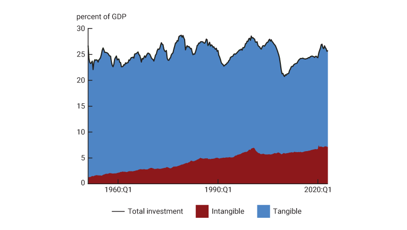
intangible investment—in gross domestic product (GDP) from 1953:Q1 through 2023:Q1. See the definitions of
tangible and intangible investment in the text.
Source: Authors’ calculations based on data from the U.S. Bureau of Economic Analysis from Haver Analytics.
Heterogeneous interest rate sensitivities
We now measure interest rate sensitivities for different components of GDP, which we also refer to as “sectors.”
Estimating interest rate sensitivities is not straightforward: Simply noting that some sectors contract more
when interest rates rise may be misleading because interest rates might be endogenous—i.e., they may be moving
in response to some other factor that is also directly affecting investment. For instance, the Federal Reserve
sets short-term interest rates to achieve its dual
mandate goals of maximum employment and low and stable inflation, so higher interest rates can simply
reflect that economic activity is strong and that the Federal Reserve believes higher interest rates
are needed to prevent higher inflation. To solve the “identification problem,” we follow Romer and Romer (2004),
who construct a series of monetary policy “shocks,” i.e., changes in interest rates that are not driven by
economic activity or inflation and, hence, are possibly independent of other factors driving investment.5 An example would be a period when the Federal Reserve decided that
it was valuable to reduce inflation regardless of current economic conditions.6
With this shock series in hand, we follow Romer and Romer (2004) and more specifically McKay and Wieland (2021)
and estimate the responses of each sector to changes in interest rates using linear regressions (“local
projections”) of the form:
$3)\quad{{y}_{t+h}}={{\unicode{x03B1} }_{h}}+\sum\limits_{m=0}^{M}{{{\unicode{x03B2}
}_{h,m}}R{{R}_{t-m}}}+\sum\limits_{l=1}^{L}{{{\unicode{x03B3} }_{h,l}}{{y}_{t-l}}+{{\unicode{x03B4}
}_{h}}t+{{\unicode{x03B5} }_{t+h}},}$
where h = 0 …16 denotes the horizon (in quarters) at which we estimate the response; yt =
log Yt (the log of) each outcome variable (e.g., tangible or intangible investment);
RRt the Romer–Romer monetary policy shocks; t a time trend; ${{\unicode{x03B5} }_{t}}$
an error term; and ${{\unicode{x03B1} }_{h}},\,{{\unicode{x03B2} }_{h,m}},\,{{\unicode{x03B3} }_{h,l}},$ and
${{\unicode{x03B4} }_{h}}$ the corresponding regression coefficients.7
We estimate equation 3 using quarterly data over the period 1969:Q1 through 2007:Q4, with M = L = 16; and
figures 2–4 depict, for various categories of spending yt, the coefficients $\left\{
{{\unicode{x03B2} }_{h,0}} \right\}_{h=0}^{H},$ which trace out the so-called impulse response function (IRF).
We normalize the impulse response so that the shock studied corresponds to a 100 basis point increase in the
real one-year U.S. Treasury rate, which is a common measure of the stance of monetary policy.
Figure 2 depicts the responses of consumption and total investment to a tightening of monetary policy (that
increases the real one-year rate by 100 basis points). The figure shows that investment is much more responsive
to a change in monetary policy than consumption: While both sectors decline in response to higher interest
rates, investment falls over 1.5% (to its nadir), with consumption decreasing less than 0.2%. To put the results
another way, the investment sector accounts for the bulk of the impact of monetary policy on economic activity.
2. Impulse responses of consumption and total investment to a monetary policy shock
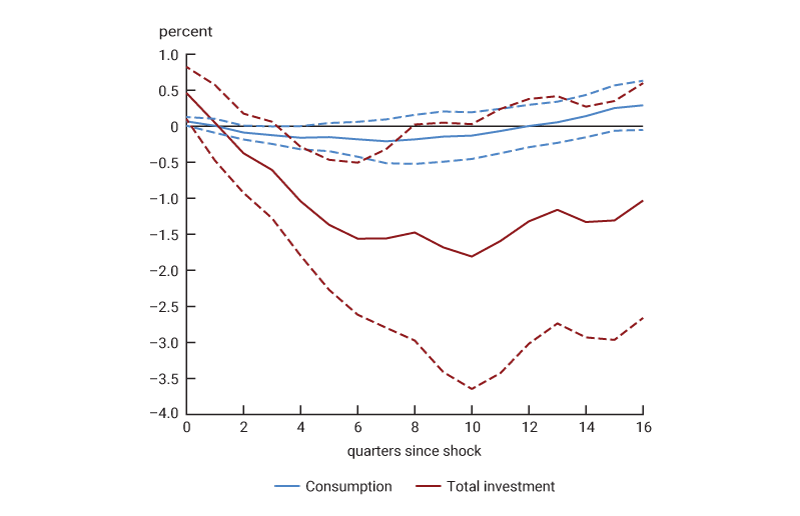
to a Romer and Romer (2004) monetary policy shock. Solid lines denote point estimates and the corresponding
dashed lines 90% standard error bands.
Sources: Authors’ calculations based on data from Wieland and Yang (2020) and the U.S. Bureau of Economic
Analysis from Haver Analytics.
Next, figure 3 depicts the responses of tangible and intangible investment to the same tightening of monetary
policy. Strikingly, tangible investment is entirely responsible for the negative total investment response. If
anything, intangible investment reacts with the opposite sign, though the magnitude of the effect is
substantially smaller than for tangible investment and is very short-lived (e.g., the response is statistically
significant for only two quarters).8
3. Impulse responses of tangible and intangible investment to a monetary policy shock
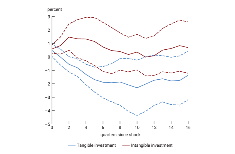
(2004) monetary policy shock. Solid lines denote point estimates and the corresponding dashed lines 90%
standard error bands.
Sources: Authors’ calculations based on data from Wieland and Yang (2020) and the U.S. Bureau of Economic
Analysis from Haver Analytics.
To understand which categories of investment are driving the result, we plot in figure 4 the estimated responses
of the components of investment defined in equation 2 to the same monetary policy shock. For ease of comparison,
all the panels in figure 4 have the same scale. Panels A and B depict the responses of the two components of
intangibles: intellectual property products and high-tech equipment. The general lack of response of
intellectual property products to the shock is noteworthy; the response of high-tech equipment is mildly
positive for two quarters and then becomes statistically indistinguishable from zero. Panels C and D plot the
responses of the two traditional investment components: equipment (excluding high-tech equipment) and
nonresidential structures. The non-high-tech equipment category responds strongly negatively to the shock, but
with a long lag; meanwhile, puzzingly, the nonresidential structures category responds positively.9 Finally, panels E and F show that residential structures are the
component of investment that responds the most negatively (and also, the fastest) and that consumer durable
spending also reacts fairly strongly negatively.
3. Impulse responses of tangible and intangible investment to a monetary policy shock
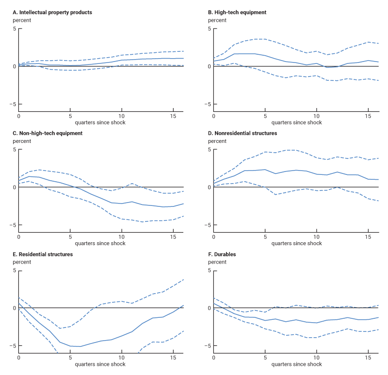
monetary policy shock. Solid lines denote point estimates and the corresponding dashed lines 90% standard
error bands.
Sources: Authors’ calculations based on data from Wieland and Yang (2020) and the U.S. Bureau of Economic
Analysis from Haver Analytics.
Estimating the change in the transmission of monetary policy
How do the changing investment shares documented in figure 1 affect the transmission of monetary policy to
economic activity? The overall percentage change in total GDP for a given change in interest rates is the sum of
the contributions of each sector; and a sector’s contribution is the product of the sector’s share in GDP and
its individual responsiveness to a change in interest rates. If each sector had the same interest rate
sensitivity, reallocation of activity across sectors would have no effect on monetary transmission. In contrast,
if sectors differ in their interest rate sensitivities, as figure 3 shows is the case for intangible and
tangible investment, reallocation toward sectors with low (high) rate sensitivities decreases (increases) the
overall responsiveness to changes in rates.10 Using the estimated
responses for each type of investment along with each type’s share of GDP, we can quantify the implications of
the changing shares for the transmission of monetary policy to overall economic activity. Figure 5 reports our
calculations. The first column displays the estimated impulse response of each investment category, e.g., the
coefficient ${{\unicode{x03B2} }_{h,0}}$ from equation 3, at a horizon h of nine quarters, which
corresponds to the peak response of GDP to the monetary shock. In panel A of figure 5, we report the 1953 and
2019 shares of each investment category in total investment and the implied contribution of each category in
each period to the rate sensitivity of total investment (calculated as the first column’s value multiplied by
second or fourth column’s value, depending on the year). In panel B, we report the analogous statistics for GDP.
5. Investment shares and monetary policy transmission
| 1953 | 2019 | |||||
|---|---|---|---|---|---|---|
| IRF (h = 9) (1) |
Share (2) |
Contribution (3) |
Share (4) |
Contribution (5) |
||
| A. Investment | ||||||
| Nonresidential structures | 2.13 | 0.14 | 0.30 | 0.13 | 0.28 | |
| Non-high-tech equipment | –2.08 | 0.20 | –0.42 | 0.15 | –0.31 | |
| High-tech equipment/IPP | 0.18 | 0.07 | 0.01 | 0.27 | 0.05 | |
| Residential structures/durables | –3.09 | 0.59 | –1.83 | 0.45 | –1.38 | |
| Total | – | 1.00 | –1.94 | 1.00 | –1.37 | |
| B. GDP | ||||||
| Nonresidential structures | 2.13 | 0.03 | 0.07 | 0.03 | 0.07 | |
| Non-high-tech equipment | –2.08 | 0.05 | –0.10 | 0.04 | –0.08 | |
| High-tech equipment/IPP | 0.18 | 0.02 | 0.00 | 0.07 | 0.01 | |
| Residential structures/durables | –3.09 | 0.14 | –0.44 | 0.11 | –0.34 | |
| Total | – | 0.24 | –0.46 | 0.24 | –0.33 | |
From the third column of figure 5, panel A, the total investment response in 1953 to a 100 basis point interest
rate shock (in terms of the real one-year Treasury rate) was –1.94%. This negative response is entirely
accounted for by the non-high-tech equipment and residential structures/durables categories. By 2019, because of
shifting investment shares alone, the fifth column shows that the total implied investment response had fallen
(in absolute value) to –1.37%—a decline of 0.57 percentage points, or roughly 30%. The result stems from the
fact that between 1953 and 2019, the share in total investment of the two most interest-rate-sensitive
categories—non-high-tech equipment and residential structures/durables—fell by about 20 percentage points, from
79% to 60% (see the second versus fourth columns), whereas the share of intangibles (high-tech
equipment/intellectual property products)—which are not sensitive to interest rates—rose by essentially the same
amount, from 7% to 27%. Figure 5, panel A shows that this change in the composition of investment may have
dampened the investment response to monetary policy by almost 30%.
Similarly, figure 5, panel B shows that changing investment shares reduced the interest rate sensitivity of
GDP—by about 0.13 percentage points between 1953 and 2019, from –0.46% to –0.33%. (Note that the compositional
effects on GDP are approximately equal to the effects on investment, scaled by the investment share of GDP,
which was 24% in both of these years.) The results imply that the rise of intangible investment may have
dampened the impact of monetary policy on overall economic activity by 27%—in other words, about
one-quarter.11
Conclusion
We have shown that the rising importance of intangibles may have dampened the responsiveness of economic activity
to changes in interest rates—by as much as one-quarter according to our estimates. This result does not
necessarily imply that the Federal Reserve has less ability to affect output than in the past; rather, it
implies that the impact of a given rate change may be smaller than in the past, so larger changes in interest
rates may be required to affect output by the same amount as before. One important assumption to keep in mind is
that the interest rate sensitivities of tangible and intangible investment have stayed constant over time. To
the extent that these sensitivities are time-varying as well, the impact of reallocation from tangible to
intangible investment could be either heightened or diminished.
But we have left open one question: Why do intangible investment and tangible investment differ in their
responsiveness to changes in interest rates? There are at least two plausible explanations.12 First, the expected lifetime of intangibles is typically shorter than that of
tangible capital; i.e., intangibles tend to depreciate faster—for example, the depreciation rate on intellectual
property is a little over 20%, compared to just over 2% for residential structures.13 This makes the cost of investing in intangibles less sensitive to interest
rates, since their payoffs are not as backloaded. Second, intangible investment appears to be financed
differently than tangible investment: Intangibles are financed primarily using internal funds or equity, rather
than through debt, likely reflecting, at least in part, the fact that tangible capital is easier to pledge as
collateral for new loans. This would naturally make tangible investment more sensitive to financial conditions
in debt markets.
Notes
1 For some recent discussions on the role of intangibles, see, e.g.,
Corrado et al. (2022), Crouzet et al. (2022), and Bronnenberg, Dubé, and Syverson (2022)—all in the Summer 2022
issue of the Journal of Economic Perspectives—and Haskel and Westlake (2018).
2 For some work on the measurement of intangibles, see Corrado,
Haltiwanger, and Sichel (2005), Corrado, Hulten, and Sichel (2009), and Lev (2001).
3 Note that we categorize consumer durables as a form of investment,
although the BEA does not.
4 It would be interesting to expand our analysis to other forms of
intangibles not yet incorporated by the BEA into the NIPAs; see, for instance, Morlacco and Zeke (2021), who
study expenditures on advertising.
5 More specifically, the Romer and Romer (2004) shock series measures
the deviations of the policy interest rate from a “rule”—i.e., it extracts movements in the (target) federal
funds rate that are unrelated to changes in Federal Reserve internal (Tealbook/Greenbook)
forecasts of future economic conditions and inflation and to the lagged federal funds rate.
6 There are of course other methodologies to estimate the effects of
monetary policy or, more broadly, the interest rate sensitivity of each sector. We use the Romer and Romer
(2004) series, which was updated by Wieland and Yang (2020), because it allows us to use a sample that aligns in
time with the secular increase in intangible capital we study. In unreported results, we obtained similar
findings using shocks identified via vector autoregression (VAR) with timing restrictions as in Christiano,
Eichenbaum, and Evans (1999).
7 In general, a regression model is a statistical method that
estimates the strength of relationships between variables. A regression coefficient represents the expected
change in the dependent variable for a one-unit change in the independent variable (while holding constant any
other independent variables).
8 Our results are consistent with the study of Döttling and Ratnovski
(2023), which uses microdata on firm investment rather than macroeconomic data.
9 Several explanations have been advanced for the erratic behavior of
nonresidential structures. First, the length of the process to plan and implement such large-scale projects may
induce a long lag. Second, there is natural substitution in the production of residential and nonresidential
structures: Construction inputs (both workers and materials) can switch between producing one or the other.
Hence, as residential investment declines, the construction industry might find it appealing to build
nonresidential structures instead.
10 Of course, these calculations assume that the interest rate
sensitivity of each sector is not itself changing. One possibility is that intangibles have become more
sensitive to changes in interest rates. Investigating whether this is the case would necessitate long enough
time-series data to robustly estimate time-varying impulse response functions.
11 To calculate this value, we use the values in figure 5 and the
shares and impulse responses of the consumption and residual categories defined in equation 1 to derive the
total response of GDP to the monetary shock of –0.49% in 1953. (Note that this value of –0.49% is quite close to
the GDP response obtained by summing the responses of investment categories, i.e., –0.46%, reported in the third
column of figure 5, panel B—which reflects that consumption and the residual, on net, contribute little to the
response of GDP.) The percentage fall in GDP sensitivity due to the rise in intangibles is then
$\frac{-0.13}{-0.49}=0.27.$
12 See also related work by Crouzet and Eberly (2019), Caggese and
Pérez-Orive (2022), and Döttling and Ratnovski (2023).
13 Authors’ calculations based on data from table 1.3 and table 1.1
of the Fixed Asset Accounts Tables of the BEA.
References
Bronnenberg, Bart J., Jean-Pierre Dubé, and Chad Syverson, 2022, “Marketing investment and intangible brand
capital,” Journal of Economic Perspectives, Vol. 36, No. 3, Summer, pp. 53–74. Crossref
Caggese, Andrea, and Ander Pérez-Orive, 2022, “How stimulative are low real interest rates for intangible
capital?,” European Economic Review, Vol. 142, February, article 103987. Crossref
Christiano, Lawrence J., Martin Eichenbaum, and Charles L. Evans, 1999, “Monetary policy shocks: What have we
learned and to what end?,” in Handbook of Macroeconomics, John B. Taylor and Michael Woodford
(eds.), Vol. 1A, Amsterdam: Elsevier / North-Holland, pp. 65–148.
Corrado, Carol, John Haltiwanger, and Daniel Sichel (eds.), 2005, Measuring Capital in the New
Economy, National Bureau of Economic Research Studies in Income and Wealth, Vol. 65, Chicago:
University of Chicago Press.
Corrado, Carol, Jonathan Haskel, Cecilia Jona-Lasinio, and Massimiliano Iommi, 2022, “Intangible capital and
modern economies,” Journal of Economic Perspectives, Vol. 36, No. 3, Summer, pp. 3–28. Crossref
Corrado, Carol, Charles Hulten, and Daniel Sichel, 2009, “Intangible capital and U.S. economic growth,”
Review of Income and Wealth, Vol. 55, No. 3, September, pp. 661–685. Crossref
Crouzet, Nicolas, and Janice C. Eberly, 2019, “Understanding weak capital investment: The role of market concentration and intangibles,” in Changing Market Structures and Implications for Monetary Policy, proceedings of the 2018 Jackson Hole Economic Policy Symposium, Federal Reserve Bank of Kansas City, pp. 87–149, available online.
Crouzet, Nicolas, Janice C. Eberly, Andrea L. Eisfeldt, and Dimitris Papanikolaou, 2022, “The economics of
intangible capital,” Journal of Economic Perspectives, Vol. 36, No. 3, Summer, pp. 29–52. Crossref
Döttling, Robin, and Lev Ratnovski, 2023, “Monetary policy and intangible investment,” Journal of Monetary
Economics, Vol. 134, March, pp. 53–72. Crossref
Haskel, Jonathan, and Stian Westlake, 2018, Capitalism Without Capital: The Rise of the Intangible
Economy, Princeton, NJ: Princeton University Press.
Lev, Baruch, 2001, Intangibles: Management, Measurement, and Reporting, Washington, DC: Brookings
Institution Press.
McKay, Alisdair, and Johannes F. Wieland, 2021, “Lumpy durable consumption demand and the limited ammunition of
monetary policy,” Econometrica, Vol. 89, No. 6, November, pp. 2717–2749. Crossref
Morlacco, Monica, and David Zeke, 2021, “Monetary policy, customer capital, and market power,” Journal of
Monetary Economics, Vol. 121, July, pp. 116–134. Crossref
Romer, Christina D., and David H. Romer, 2004, “A new measure of monetary shocks: Derivation and implications,”
American Economic Review, Vol. 94, No. 4, September, pp. 1055–1084. Crossref
Wieland, Johannes F., and Mu-Jeung Yang, 2020, “Financial dampening,” Journal of Money, Credit and
Banking, Vol. 52, No. 1, February, pp. 79–113. Crossref


Leave a comment